

We had sized prod from Camunda’s reference architecture and our own arithmetic. No real load had passed through it. We spent the next week finding a capacity number we could support with measurements.
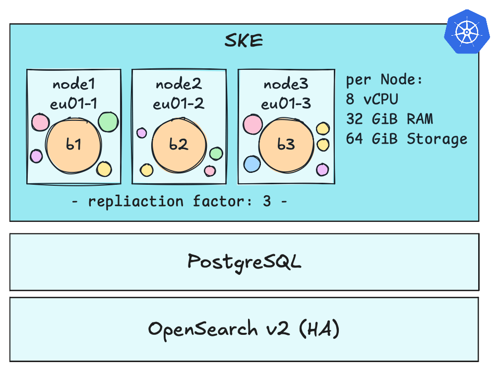
The prod setup under test had three g2i.8 nodes, 8 vCPU and 32 GiB each, one per availability zone, with Zeebe across them as three brokers, three partitions, replication factor 3 and a 64 Gi volume per broker. Secondary storage is a managed OpenSearch service, three nodes in HA, which started the week at 2 vCPU and 8 GiB per node. Two exporters run on every partition: the newer one feeds Operate, Tasklist and the search APIs, and the legacy one is there because Optimize needs it.
The first graph looked good. For a few minutes we thought the platform had exceeded our expectations, until the job-completion count showed that the generator was producing far less load than configured. Later runs repeated that pattern: one metric supported a capacity estimate, then another showed which limit we had measured. Across six runs, we produced four estimates and discarded three.
Note: The bench cluster is specific to our setup. The measurement errors apply to any Camunda 8 benchmark.
How Camunda Absorbs Load
Camunda absorbs load by measuring itself. Nothing here caps the request rate. Each broker derives its own ceiling from how fast it is answering, and three loops move that ceiling.
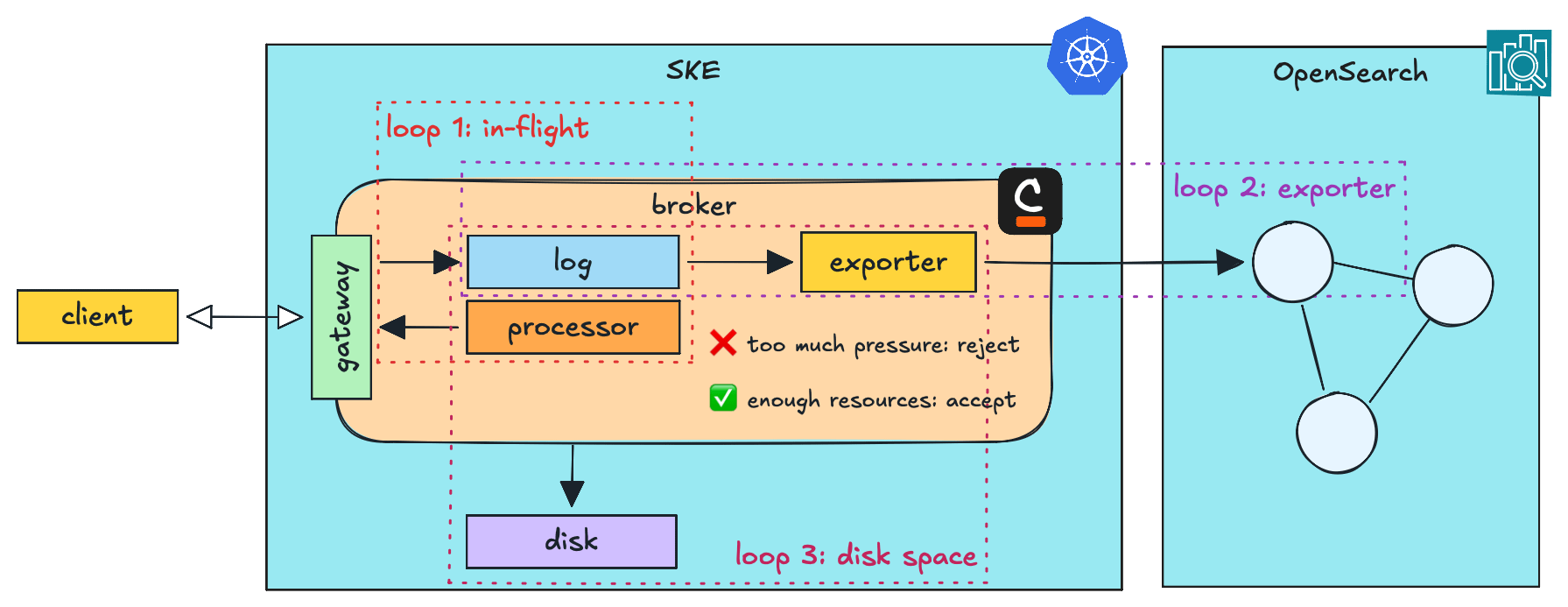
The first loop: A command is not executed when it arrives. The broker appends it to its partition’s log, and the stream processor reads it back later. So a broker always holds requests it has accepted and not yet answered. It counts those, in flight, and measures the round trip from accepting a request to answering it. Above a limit on the in-flight count, requests are rejected instead of queued. That rejection is backpressure, and limit and count are both per partition.
The limit moves. An adaptive algorithm recalculates it, AIMD by default: a round trip faster than the broker expects raises the limit by one, a slower one cuts it by a tenth. Ours sits at an initial 100 in-flight / partition, with a floor of 1 so sustained load cannot walk it down to nothing.
Exporters close the second loop. Each walks the same log from its own position into secondary storage, the copy that Operate, Tasklist, Optimize and the search APIs read. Flow control limits the export write rate too, and can throttle it as the unexported backlog grows. Slower writes leave the stream processor waiting on its results, the round trip lengthens, the limit shrinks. A slow search cluster reaches clients as engine backpressure.
Disk closes the third loop. The log compacts only up to the earliest exporter position, so an exporter that stops advancing keeps it growing. Below 2 GB free the broker rejects every client command and pauses processing, and below 1 GB it stops accepting replicated events too. Both limits can be configured.
Whichever loop closed, the client gets RESOURCE_EXHAUSTED over gRPC, or an HTTP 503 saying the same, and should retry with backoff and jitter. A flood of start requests and a slow OpenSearch look identical from out there. Completing and failing a job are exempt, accepted above the limit, because work already inside has to be able to leave.
The First Run Measured The Client
We use the camunda-8-benchmark project from Camunda Community Hub to put load on prod. It starts process instances at a configured rate and completes the service tasks in the synthetic model.
The pilot started from a laptop, with one generator driving prod over the public gRPC path at 150 process instances per second. The first dashboard looked almost too good: backpressure stayed under 1%, with no engine ceiling in sight. We wanted to believe the sizing had headroom.

The job-completion count showed the problem. The model has ten sequential service tasks, so 150 PI/s needs roughly 1.500 completions per second. The generator plateaued between 585 and 606. We traced the gap to the ingress recycling HTTP/2 connections after about a thousand requests. Each recycle killed the job-push streams, leaving pushed jobs on dead streams until timeout. Prod had looked comfortable because it never received the load we thought we were sending.
So we built a permanent cluster whose only job is generating load: three nodes, one generator per node so they cannot contend for a CPU or a network queue. Generators inside prod would have been cheaper and wrong twice, because their CPU competes with the brokers and they skip the public ingress path under investigation. The bench cluster comes in over the internet instead, admitted by a narrow allowlist on that one route.
Every run since reports the generators’ own CPU against their limit. Peak draw went from 868 millicores on the first cluster run to 98 of a 3.000 limit on the last. A load test that cannot show its generator had headroom has not established what it measured.
The Bottleneck Was Downstream
With three generators, we offered the same 150 PI/s aggregate and watched the client path stay clean: zero GOAWAY, zero closed streams, zero UNAVAILABLE. Prod now received the intended load. Every error was engine-side, and backpressure reached 42% of start attempts against a 10% target.
The engine was only one path. Export lag climbed on all three partitions to 2,85 million records after five and a half minutes of load, and draining it afterwards took fourteen minutes. The original sizing exported about 280.000 records per minute, so every minute of load cost roughly 2,5 minutes of export tail. Export capacity, not the engine, bounded how long a run could last. Both sides of that ratio changed again later in the week.
We answered with three changes at once. That got the next run moving and made attribution impossible. Each broker went from a 2 Gi memory request and a 4 Gi limit to 4 Gi and 8 Gi, with its CPU limit left at 3 cores. The managed search cluster moved from three nodes at 2 vCPU and 8 GiB to three at 4 vCPU and 16 GiB. We also set the exporter’s index refresh interval to 5 seconds. Together they raised export capacity about 36%, to 380.000 records per minute.
The broker resize added memory headroom. Peak working set stayed at 3,73 GiB, which was 91% of the old limit and 47% of the new one. Because the image exits the JVM on out-of-memory, a longer run at the old limit could have cost us quorum.
Capacity Arithmetic Uses The Accepted Rate
Export remained the bottleneck, so we wanted the rate at which its backlog stopped growing. Two reports estimated that rate instead of measuring it, and both came out about 2,4 times too high.
The method was reasonable. Export capacity and record generation are both rates, so dividing one by the other tells you what share of the current load the exporter can keep up with. Apply that share to the load and you have a sustainable rate.
The load we applied it to was the wrong number. We’re offering 150 process instances per second, but backpressure was rejecting 40 - 47% of those starts, so the engine only ever accepted around 80. Nearly half the load in the calculation never reached the engine.
Capacity arithmetic has to use accepted starts. Nothing in the tooling tells you which of the two rates you are looking at, so it is worth checking before either one goes into a calculation. Once we saw the mistake, another spreadsheet felt less useful than a measured crossing point, so we went back to the cluster.
Backpressure Is Not A Capacity Signal
Sustainable means export lag neither grows nor shrinks over a long window, measured as the slope of the lag curve. We kept a standing backlog between steps instead of draining, so the exporter stayed saturated and the slope was generation minus capacity. Draining between steps would have made every slope depend on the exporter warming up again.
# Export lag: positions appended to the log, minus positions the exporter
# has walked. Take the slope over a long window; the level tells you nothing.
sum(
    max by (partition) (zeebe_log_appender_last_appended_position)
  - max by (partition) (zeebe_exporter_last_exported_position)
)
We planned to increase the rate in fixed steps from 75 PI/s. The first step produced +415,000 records per minute of lag, so we reduced the rate instead. Four steps at 75, 45, 36 and 30 PI/s gave lag slopes of +415.000, +118.000, +2.000 and −85.000 records per minute. The line between them crossed break-even at 35,9 PI/s.
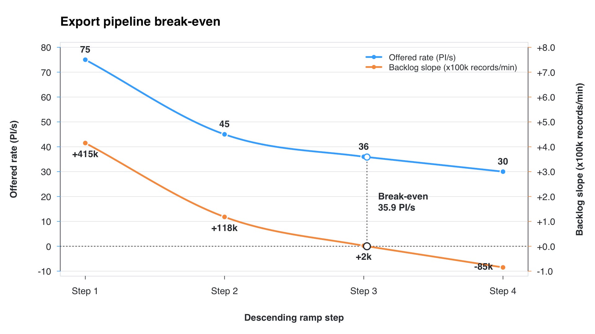
Backpressure was useless as the instrument. At 30, 36 and 45 PI/s it sat at zero while export fell behind by up to 118.000 records per minute. The benchmark tooling’s ramp strategies climb until the engine pushes back, so they would have reported double the truth. Export capacity itself was a hard constant near 427.000 records per minute, within 0,4 % whether the brokers were under full load or idle. Nothing was bought between that and the 380,000: same brokers, same plan, one drain reading in an earlier run against a saturated exporter here.
The Cheapest Capacity Was Free
The largest improvement was already available in the exporter configuration. The legacy exporter serialized everything the engine produced even though Optimize, its only consumer, imports five record types.
Cutting the job records alone, 18% of that exporter’s write volume, had bought no throughput at all, because the metric that bounds run length counts log positions walked rather than documents written. What worked was dropping records before serialization instead of after, with the exporter’s own filter for what Optimize imports, plus skipping a class of variable writes on the newer exporter. Same hardware, same load profile, one configuration change:
export capacity from 427.000 to at least 851.000 records per minute, a measured 2x, with 40% of the exporter thread still idle
the post-run drain from 2,68 million records and nearly nine minutes to 26.000 records and about 90 seconds
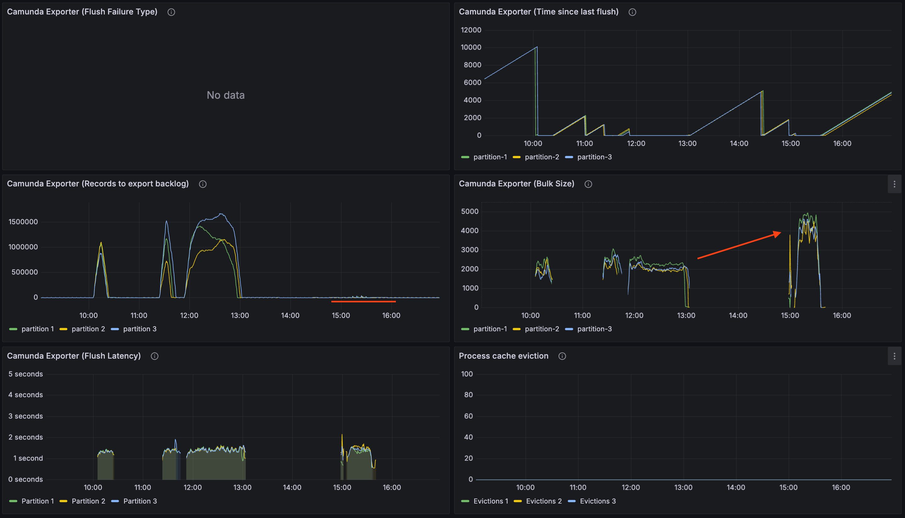
We had bought hardware before finding the configuration limit. The larger plan raised capacity 1.36x and added a permanent monthly charge; the filter doubled it on the machines already running. The upgrade was still useful because it doubled the search cluster’s heap, and shard count has since outgrown what the old plan could hold. We should have finished reviewing the exporter configuration before upgrading the search plan. Part 6 shows the cost.
What It Holds
Doubling export capacity also doubled the projected break-even rate. The 35,9 PI/s result belonged to roughly 427,000 records per minute of export; at 851.000, the calculated balance is near 72 PI/s. At that rate, engine acceptance became the limiting factor. On the final run we increased the offered rate again, with export tracking generation at every step.
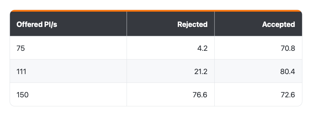
On the final run, accepted throughput peaked around 80 process instances per second and fell to 72.6 when we offered nearly twice that, because rejecting a start still costs the engine work. We trust the range of 72 to 80 accepted process instances per second at this broker CPU limit, with no connectors. Prod completed 963,902 jobs across 25 minutes of load. One instance of this model produces ten jobs and about 186 log records, and that second number is the conversion to redo before comparing any of this to a different process.
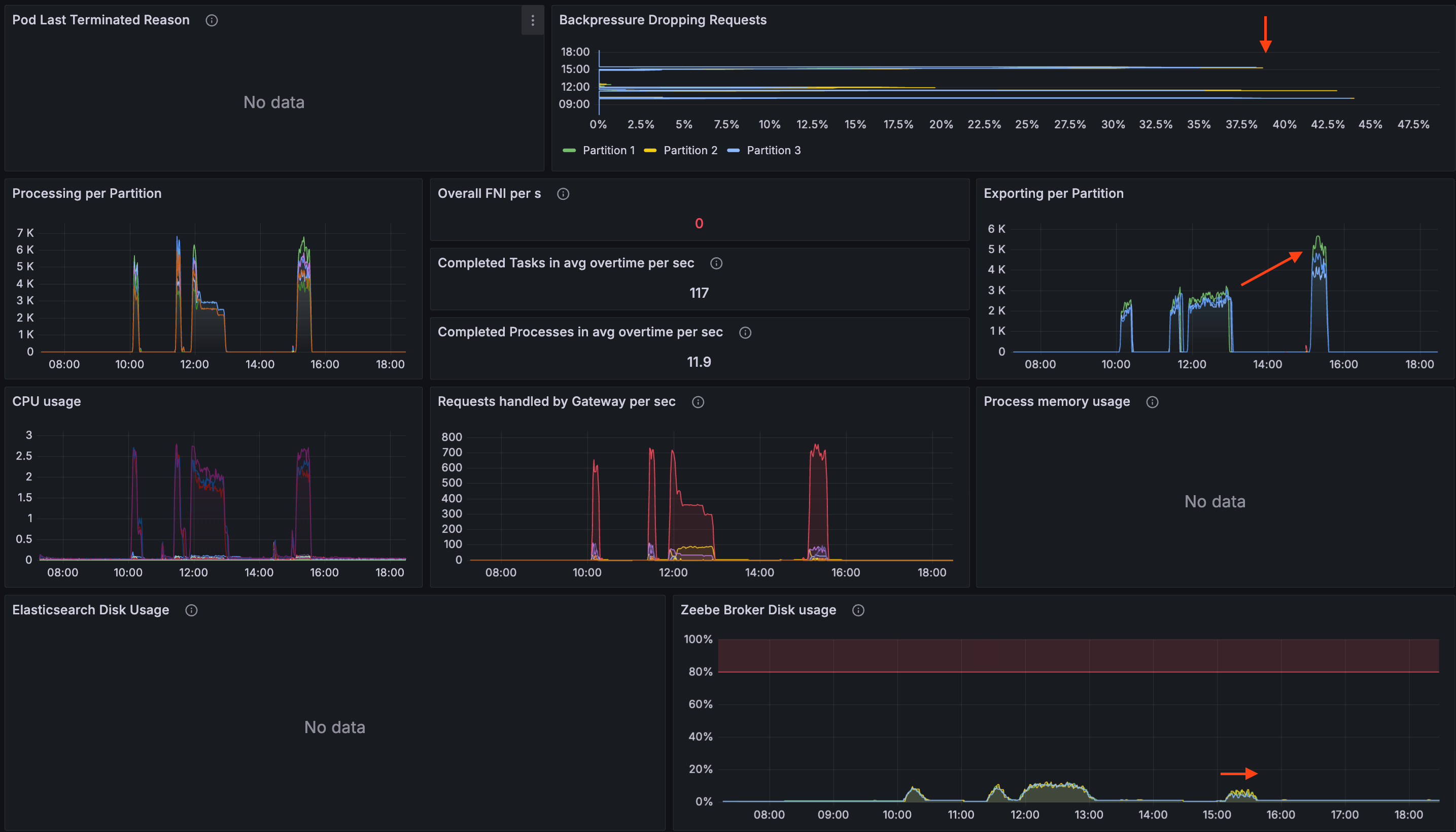
That ceiling is self-imposed. Each broker runs with a CPU limit of 3 cores, sat at 2,7 of them under load, and spent 27 to 48% of its scheduler periods throttled against that limit. The nodes underneath have 8 vCPU, and the busiest of the three peaked at 2,7 cores of the 7,9 it has to give. We set the limit to cover the broker’s three processing threads and left the request at 1 core, because that busy node also carries the ingress controllers and every non-broker Camunda component and is already at 79% of its CPU requests. The measured ceiling belongs to those resource limits; raising them remains untested.
The relevant alert changed with the bottleneck. Export backlog identified the limit in the middle runs while backpressure stayed silent. After the exporter change, backpressure identified the engine limit and export lag stayed flat.
Operate and the v2 search and statistics APIs read the secondary store, which in the early runs still reported ten thousand active instances more than an hour after everything had finished. Ground truth is the broker’s exported position. Never diagnose engine state from the search APIs under load.
The process shape is synthetic, ten sequential service tasks and two timer catch events, not a customer’s mix. The longest window we held flat was 22 minutes and the final run carried 25 minutes of load, so nothing here says what a day of it does. We also measured throughput and not client response time, so how long a start takes to return at 70 PI/s is still an open question.
What You Turn If You Need More
If you need more throughput, start with the broker CPU limit because the nodes already have unused capacity. Whether raising it moves the accept ceiling is untested: append rate held flat near 13.500 records per second across all three steps of the final run, which does not look CPU-bound, so change one variable and measure. The next option is more cores per broker or bigger nodes, both of which add a permanent cost. More partitions provide horizontal scale, but raising the partition count is a one-way door.
Whichever lever you pull, export has to move with it. Its capacity is a hard constant for a given configuration, and break-even scales with that constant. Raising the accept ceiling alone relocates the bottleneck.
What’s Next
The number that survived six runs is 72 to 80 accepted process instances per second at this sizing. The method is what carries beyond our setup: measure the accepted rate and never the offered one, read the export backlog slope while export is the bottleneck, and find out what the exporter thread is doing before buying hardware.
Part 6 closes the series with the bill: what the platform costs to run, what held, what hurt, and whether the sovereignty trade was worth it.